(Equation 9.7)
Although a handful of isolated recombinant inbred (RI) mouse strains were developed during the 1940s and 1950s, the importance of these genetic constructs was not appreciated by any scientist prior to Dr. Donald Bailey who first conceptualized their potential utility for linkage analysis while working at the National Institutes of Health in 1959 (Bailey, 1981). Bailey realized that established sets of RI strains could provide an efficient alternative to the lengthy process of classical breeding analysis that was required at that time to map any newly uncovered locus. Bailey moved with his first set of eight RI strains — the original CXB set — to the Jackson Laboratory in 1967. In 1969, Dr. Benjamin Taylor, also at the Jackson Laboratory, took up the cause of the RI approach and set about developing, from several different pairs of progenitor parents, large sets of RI strains that are now standards for the mouse genetics community including BXD, BXH, AKXL and AKXD (Taylor, 1978; Table 9.3). These standard RI sets, and others listed in Table 9.3 under JAX availability, can be purchased directly — in the form of either animals or DNA — from the Jackson Laboratory. Today, recombinant inbred strains represent a critical tool in the arsenal used to map mouse genes and the RI approach has made its way into the study of other experimental organisms as well such as the plant Arabidopsis (Lister and Dean, 1993).
The construction of a set of RI strains is quite simple in theory and is illustrated in Figure 9.4. One begins with an outcross between two well-established highly inbred strains of mice, such as B6 and DBA in the example shown. These are considered the progenitor strains. The F1 progeny from this cross are all identical, and thus in genetic terms, they are all interchangeable. F1 hybrid animals are bred to each other to produce a large set of F2 animals. At this generation, siblings and cousins are no longer identical because of the segregation of B6 and DBA alleles from the heterozygous F1 parents. As illustrated in Figure 9.4 for a single pair of homologs, each of the F2 animals will have a unique genotype with some loci homozygous for the B6 allele, some homozygous for the DBA allele, and some heterozygous with both alleles. At this stage, pairs of F2 animals are chosen at random to serve as the founders for new inbred strains of mice. The offspring from each F2 founder pair are maintained separately from all other offspring, and just two are chosen randomly for brother-sister mating to produce the next generation. The same process is repeated at each subsequent generation until at least 20 sequential rounds of strict brother-sister matings have been completed and a new inbred strain with special properties is established. 75
Each of the new inbred strains produced according to this breeding scheme is called a "recombinant inbred" or "RI" strain. Different RI strains produced from the same pair of progenitor strains are considered members of the same "RI set." Each RI strain is named with an uninterrupted string of uppercase letters and numbers that can be broken down into the following components: (1) a shortened version of the maternal progenitor strain name; (2) the uppercase letter "X"; (3) a shortened version of the paternal progenitor strain name; and (4) a hyphen and a number to distinguish each strain from all other strains in the same RI set. 76 The first three components of an RI strain name are also used alone as the name for the corresponding RI set.
Table 9.3 lists the 17 RI sets that have been used to a significant degree by members of the mouse genetics community (R.W. Elliott, personal communication). The most readily available of these are the ones that can be purchased directly from the Jackson Laboratory (JAX) in the form of live animals or DNA — fourteen RI sets with a total of 187 strains. The best-known and most well- characterized RI set is BXD with 26 extant strains formed from an initial cross between B6 females and DBA/2J males. Individual strains within this set are called BXD-1, BXD-2, BXD-5 and so on. (The BXD-3, BXD-4 and other missing strains are now extinct and their numbers have been retired.) By August of 1993, 818 loci had been typed on the BXD set. Unfortunately, as discussed earlier in this book (Sections 2.3.4 and 3.2.2), the two progenitors of the BXD set — B6 and DBA — are related to each other through the common group of founder animals used to develop most of the classical inbred strains at the beginning of the twentieth century. As a consequence, a significant number of loci will show no variation between the two progenitors even with highly sensitive PCR protocols that detect SSCPs and microsatellites (see Section 8.3).
More recently, two progenitor mouse strains — A/J and C57BL/6J — known to differ in susceptibility to over 30 infectious or chronic diseases were used to establish a new pair of RI sets — AXB and BXA — based on reciprocal crosses (Marshall et al., 1992). Genetic surveys suggest that these progenitors are much less related to each other than B6 is to DBA, and with 31 genetically validated extant strains 77 available from the Jackson Laboratory, this paired set is the largest, and likely to be the most useful for both linkage analysis and the study of complex traits that differ between the two progenitors.
At any time, it is possible to add to the numbers of strains in a particular RI set by starting from scratch with a new cross between the original progenitor strains and following it through twenty generations of inbreeding. In this manner, J. Hilgers at the Netherlands Cancer Institute in Amsterdam and L. Mobraaten at the Jackson Laboratory have increased the size of the original CXB RI set with five and six new strains, respectively.
Like all inbred strains, RI strains are fixed to homozygosity at essentially all loci. 78 Thus, the genomic constitution of each strain can be maintained indefinitely by continued brother-sister matings, and the strain can be expanded into as many animals as required at any time. However, unlike the classical inbred strains, the genotype of an RI strain is greatly circumscribed. First, there are only two choices for the allele that can be present at each locus: thus, for every locus in every strain of the BXD RI set, only the B6 or the DBA allele can be present. Second, because there is only a limited number of opportunities for recombination to occur between the two sets of progenitor chromosomes before homozygosity sets it, complete homogenization of the genome can not take place. An illustration of this principle can be seen in Figure 9.4. In this hypothetical situation, one can see genomic regions that are already frozen at the outset of the F2 intercross in two of the three incipient RI strains. The two fixed regions are circled and (in this illustrative example) are both homozygous for B6 genomic material in the two F2 parents that will act as founders for the new BXD-102 and BXD-103 strains. At each subsequent generation, additional regions will become frozen in either a B6 or a DBA state. After 20 generations of inbreeding, each RI strain will be represented by a group of animals that will all carry the same genomic tapestry with random patches from each of the two progenitors, as illustrated in the final row of Figure 9.4.
It is this homozygous patchwork genomic structure that is the key to the power of the RI strains. This is because the boundaries that separate all of these genomic patches represent individual recombination events that are also permanently frozen. Every RI strain has different recombination sites distributed randomly throughout its genome. Thus, a set of RI strains can be used in essentially the same manner as the offspring from a mapping cross to obtain information on linkage and map distances. Like other mapping panels, it is only necessary to type each RI genotype once for a particular locus, and the information obtained from typing different loci is cumulative. The major difference, of course, is that the particular genotype present within each RI strain can be propagated indefinitely whereas different offspring from a mapping cross will all have unique genotypes and finite life spans. Thus, there is no limit to the number of loci that can be typed within an RI strain. Furthermore, in the case of complex phenotypic variation, one can actually sample the same genotype multiple times to demonstrate instances of incomplete penetrance or variable expressivity as discussed in Section 9.2.5.
The major use of RI strains by mouse geneticists today is as a tool to determine linkage and map positions for newly derived DNA clones. As the first step in this process, an investigator should survey the progenitor strains for all the most useful RI sets to determine which of these sets can be typed for the presence of alternative alleles. The strains to be surveyed should include AKR/J, DBA/2J, C57L/J, A/J, C57BL/6J, C3H/HeJ, BALB/cJ, NZB/B1NJ, SM/J and SWR/J (see Table 9.3). If one is trying to map a newly cloned gene, it is possible to start a polymorphism search based on the detection of RFLPs among DNA samples digested with one of several different enzymes (Section 8.2). However, as discussed at length in Section 8.3, one is much more likely to uncover polymorphisms with a PCR-based protocol like SSCP. 79
Once alternative alleles at a locus have been distinguished for the progenitors of any RI set, one can proceed to type all of the strains in that set. The information obtained from such a single locus analysis will represent the strain distribution pattern, or SDP, for that particular locus. An isolated SDP in and of itself is usually not informative. One would expect approximately half of the strains typed to carry each of the progenitor alleles at random. 80 However, with a new SDP in hand, it becomes possible to search for linkage with each of the other loci previously typed in the same RI set or group of sets. This is most easily accomplished with a computer program such as Map Manager that compares the new SDP to each previously-determined SDP in the database, one-by-one, and applies a statistical test for evidence against or in favor of linkage (Manly, 1993 and see Appendix B for further information).
The result of each pairwise comparison of SDPs is expressed in terms of the degree, or level, of concordance and discordance. When a particular RI strain has alleles from the same progenitor at two defined loci, the loci are considered to be "concordant" within that strain. When the alleles at the two loci come from the two different progenitors, they are considered to be "discordant". The probability of discordance is a function of the linkage distance that separates the two loci under analysis. This is easy to understand in terms of the likelihood that two loci will be retained, by chance, within the same genomic patch as illustrated in Figure 9.4. At one extreme, unlinked loci — which can not possibly lie in the same genomic patch — will be just as likely to have alleles from the same progenitor, by chance, as from the two different progenitors. Thus, one would predict that ~50% of the strains within an RI set will show concordance for a pair of unlinked loci. At the other extreme, loci that are very closely linked will always be in the same genomic patch, which is equivalent to saying that 100% of RI strains will show concordance (or 0% will show discordance). Between these two extremes will be loci that are linked, but less closely so. As the distance between two loci increases, the probability of discordance will increase in a calculable manner from 0% up to 50%.
Whenever one accumulates data on multiple RI strains, it is useful to express this information in terms of concordance and discordance rather than in terms of actual genotypes. The terms N and i are used, respectively, to denote the total number of strains typed and the number of discordant strains observed. The fraction R hat = i/N is used to denote the observed level of discordance. With the use of these terms, one can combine the data obtained from all sets of RI strains that show variation between progenitors for both loci under analysis. This can be accomplished even if different allele pairs are present in different RI sets. For example, at the H-2K locus, B6 has a b allele, DBA has a d allele, and AKR/J and A/J both have a k allele; even so, one can still combine H-2K data obtained from the BXD, AKXD, and AXB/BXA RI sets. If these three RI sets also show progenitor variation at another locus thought to be linked to H-2K, then one can count up the number of strains discordant between these two loci (i) and divide by the total number of strains (N = 82) to obtain the observed discordant fraction R hat. When strains from multiple RI sets are combined for analysis in this manner, they will be referred to as an "RI group." Increasing the size of the RI group can have dramatic effects on the sensitivity and resolution with which it is possible to determine linkage and map distances, as described in the following subsections and depicted in Figure 9.5 and Tables D1 and D2 in Appendix D.
What degree of concordance between two SDPs is required to demonstrate linkage? The problem of distinguishing a chance fluctuation above the 50% concordance expected with unlinked loci from a significant departure indicative of linkage was discussed in more general terms earlier in this chapter. Suffice it to say here that prior to 1986, researchers did not fully appreciate the more stringent requirements imposed by the Bayesian statistical approach and were misled by concordance values that passed traditional Chi-squared tests for significance. Mathematical formulations aimed at rectifying this situation were begun by J. Silver (1986) and were supplemented by Neumann (1990; 1991). In his 1990 paper, Neumann published tables with a complete set of maximum discordance values (i) that are allowed for a demonstration of linkage at various levels of significance with data obtained from RI groups up to N = 100 in size. Data from these tables have been extracted and shown graphically in Figure 9.5.
With the maximum allowable discordant values that have been determined, it is possible to estimate the maximum distance over which linkage between two loci is likely to be demonstrated at a sufficient level of significance with an RI group of a particular size. This is a measure of the "swept radius," which is a concept first developed by Carter and Falconer (1951). The swept radius has been defined as the length of a chromosome interval on either side of a marker locus within which linkage can be detected with a certain level of significance. Although the swept radius was originally defined in terms of map distance, it can be readily converted into a measure of recombination fraction (with the use of an appropriate mapping function as described in Section 7.2.2.3), which is more useful for direct analysis of raw data. In this way, the swept radius can be viewed as a boundary value for the recombination fraction. If the observed rate of recombination between two loci is less than the swept radius, linkage is demonstrated at a level of significance equal to or greater than the cutoff value chosen. If the observed rate of recombination is greater than the swept radius, linkage cannot be demonstrated with the available data. 81
The maximum discordance values allowed for each value of N can be translated into linkage distances (through the use of the Haldane-Waddington equation described in the next section) that describe swept radii at which linkage can be detected with a significance level of 95% or 99%. 82 With just 20 RI strains, one will only be likely to detect linkage with marker loci that are within 2 cM on either side of the test locus. The swept radius increases steadily as the size of the RI group climbs to 40 strains, where it becomes possible to detect linkage to markers that are within 7-8 cM of the test locus. However, even with an RI group of 100 strains, the swept radius is only 13-15 cM. In general, the distance swept by each marker locus in an RI group is only 40%-45% of the distance swept by each locus in a linkage analysis performed with an equivalent number of backcross offspring (see Figure 9.13). This disadvantage is offset by the easy availability of the major RI sets and the ever-accumulating number of marker loci for which SDPs have been determined as discussed further below.
From the preceding discussion, it should be clear that the chances of success in using RI data to demonstrate linkage for a test locus increase dramatically with both the number of strains analyzed and the number of evenly distributed SDPs that are already present in the database. As of 1993, several RI sets had been typed at over 200 loci (Table 9.3), which, if randomly distributed, would fall on the linkage map at average distances of 7 cM or less from each other. The BXD set alone has been typed for over 800 loci. Even though these marker loci are not randomly distributed, 83 their overlapping "swept diameters" of coverage are sufficient to map most new loci that are typed among all members of this set. Furthermore, RI mapping panels become ever-more efficient at detecting linkage as each new SDP is added to the database. At some point in the near future, it is likely that SDPs will be determined for all 26 BXD strains at marker loci distributed across the genome at a maximum interlocus distance of 5 cM. At this point, every new test locus of interest will have to lie within 2.5 cM of a previously-typed marker locus, and thus, by simply typing the 26 BXD strains, one will be able to determine a map position with essentially 100% probability.
Until the scenario just described is reached, it is best to maximize one's chances of demonstrating linkage by generating an SDP for the test locus over the maximal number of RI strains possible. Once data have been obtained and entered into a computer database, the first attempt to demonstrate linkage should be pursued at the highest stringency possible [equivalent to a Bayesian probability level of 99% in the Manly (1993) Map Manager program]. This will minimize the chance of picking up false linkages; if a positive result is obtained from such an analysis, one can confidently move on to the next task of determining a map position for the locus relative to the linked marker loci, as described in the next subsection. However, if this analysis fails to detect linkage, the stringency can be reduced further by small levels of significance in subsequent runs. A positive result obtained at a lower level of significance should be considered tentative and must be confirmed (or rejected) by incorporating more RI strains into the pairwise comparison between the test locus and the putatively linked marker locus, or through an independent approach such as somatic cell hybrid analysis (Section 10.2.3), in situ hybridization (10.2.2), or a backcross or intercross mapping panel (Sections 9.3 and 9.4). Independent confirmation of just the chromosomal assignment alone, for example, can serve to increase dramatically the significance level for an RI-based determination of linkage to a particular locus on that chromosome (Neumann, 1990). Furthermore, the failure to detect linkage to many markers distributed over large regions of the genome can provide evidence for the exclusion of the test locus from these other regions. This information, in turn, can be used to increase significance levels in cases where the direct evidence in favor of linkage is somewhat weak (Neumann, 1990).
In some cases, further evidence for, or against, linkage can also be obtained by comparing the SDP of the test locus to the SDPs associated with the two marker loci that putatively flank it on either side (Neumann, 1991). If the positioning of the test locus between the flanking loci is correct, one would expect to see mostly single recombination events among the three loci within individual RI strains. If the association of the test locus with this genomic region is false, one would expect to see a substantial number of double recombination events that separate the test locus from both markers. This type of analysis is most easily visualized in the form of a data matrix, discussed just below and illustrated in Figure 9.6. It is important to point out, however, that interference does not operate in the formation of RI strain genotypes since the crossover events that produced each patchwork genome occurred over multiple generations. Thus, true double recombination events over short distances are not strictly forbidden; they are just less likely.
Once linkage has been demonstrated among three or more loci, one can move on to the next step of determining their order along the chromosome relative to each other. This can be accomplished computationally with a program like Map Manger (Manly, 1993), but it is also possible to carry out this analysis without a dedicated computer program. The first task is to set up an adjustable 2 x 2 data matrix of the kind illustrated in Figure 9.6. This sample data matrix contains a subset of the actual data obtained with Chr 17 loci typed on the 26 RI strains present in the BXD set. Each row represents an independently determined SDP for the locus indicated at the left. Each column represents the complete genotype determined for an individual RI strain over the ~32 cM region that encompasses the loci shown. It is customary to order loci in the data matrix with the centromeric end of the chromosome at the top and the telomeric end at the bottom, when this information is known from other results.
A new data matrix can be initiated for any set of SDPs that have been shown to form a linkage group. It is also possible to expand an established data matrix of marker loci with the inclusion of new test locus SDPs. At the outset, SDPs can be placed into the data matrix according to a first best guess of their genetic order relative to each other. If data are entered into a computer spreadsheet, one should manually shift the order of SDP-containing rows until an arrangement is found that minimizes the total number of recombination events within the whole data set. In addition, instances of triple recombination events over short distances in individual strains should be eliminated if possible. In this manner, it is often possible to arrive at an undisputed order for an extended series of loci as is the case, for example, with the eight loci from D17Leh119 to D17Leh12 and the eight loci from D17Leh173 to D17Leh23 shown in Figure 9.6. The computer program Map Manager will carry out this process automatically and will also allow manual adjustment of order when this is desired.
There will sometimes be cases where two or more different orders appear equally likely. For example, in Figure 9.6, one could remove the Glo1 and Pim1 loci from the position shown and place them instead between H2M2 and D17Leh173. Both placements require an unsightly triple crossover: in the position shown in the Figure, this occurs in strain BXD-12; in the new genetic position, this would occur in BXD-27. Both placements also require an equal number of recombination events so it is not possible to choose one order over the other based on the BXD data alone. In this case, other mapping data have been used to confirm the map order shown in the Figure.
In general, determining map order with accuracy is increasingly more difficult with linked SDPs that are increasingly more discordant relative to each other. Increased discordance is indicative of increased interlocus distances, which make it more likely that multiple recombination events will have occurred along individual chromosomes; these will complicate the analysis. However, as is the case with all aspects of RI analysis, the more strains that are typed, the more accurate order determinations can become. For example, if SDP data obtained from the AKXL RI set had been considered in conjunction with BXD data, they would have provided unambiguous evidence in favor of the correct placement of Glo1 and Pim1 proximal to Crya1, as shown in Figure 9.6.
With the accumulation of large numbers of RI SDPs and a comprehensive two by two analysis for linkage, it becomes possible to build linkage maps that span many loci distributed over large chromosomal regions as illustrated in Figure 9.6. By looking down any column, one can clearly see the genomic patches that derive from each of the two progenitor strains. At one extreme, four strains — BXD-2, BXD-12, BXD-18 and BXD-25 — appear to have fixed three separate crossover sites in their genomes leading to the presence of four alternating B6 and DBA genomic patches. At the other extreme, 12 strains — including BXD-1, BXD-8, and ten others — appear to have inherited this chromosomal region intact, without recombination, from either the B6 or DBA progenitor. 84 The remaining ten strains have fixed either one or two crossover sites leading to two or three genomic patches respectively.
Through the visualization of RI data in this way, one can pick up suspicious results that may be due to experimental error. For example, the presence of a B6 allele at the Upg-1 locus in BXD-22 requires a double crossover that encompasses only this locus and no others. One would be advised to go back and retype this locus on a new sample from this RI strain.
By looking horizontally across the data matrix and comparing pairs of SDPs, one can visualize the degree of concordance that exists between nearby loci. At three separate junctures — D17Leh12/ Glo-1, Tpx-1/ Iapls1-3, and Ckb-rs2/ Hprt-rs1, the BXD RI data alone are not sufficient to demonstrate linkage according to the limits shown in Figure 9.5; in all these cases, data from other mapping experiments provided evidence of linkage between two or more loci present on opposite sides of these junctures. There are also numerous examples of loci that have the same SDP; as described in the next section, loci with shared SDPs across only 26 typed strains can actually be quite distant from each other in terms of map distance (see Figure 9.8).
The data matrix for this portion of Chr 17 also illustrates how the power of the RI approach to linkage determination increases with the number of loci that are typed. For example, the SDPs for D17Leh119 and Hba-ps4 are distinguished by four discordant strains (BXD-2, BXD-18, BXD-21, and BXD-25). Thus, according to Figure 9.5, these data alone do not provide sufficient evidence for linkage between these two loci at the 95% significance level. However, when the Plg SDP was added to the database, it provided the required evidence for linkage of D17Leh119 to Hba-ps4 through their common linkage — with 99% significance — to the newly typed locus.
As alluded to earlier in this section, when two loci are known to be linked, the level of discordance that is observed between their SDPs can be equated with a mean estimate of the distance that separates them. In fact, this distance estimate can be made even in those cases where the RI data alone are not sufficient to provide evidence for linkage. Thus, RI data are useful for estimating recombination distances between loci that have been linked by non-breeding methods such as physical mapping or cytogenetic analyses. However, it is not sufficient to simply determine the fraction of strains that show discordance and use this directly as an estimate of the recombination fraction. The problem is that during the generation of each RI strain, an average chromosomal region will have multiple opportunities to recombine as it passes through several generations in a heterozygous state (see Figure 9.4).
Interestingly, long before the conceptualization of RI strains,
Haldane and Waddington (1931)
derived a mathematical solution to this problem in the context
of determining the probability with which a recombinant genotype would become
fixed after successive generations of inbreeding. This solution was formulated in the
following equation where r is the probability of recombination in any one gamete
and R is the fraction of RI strains that are predicted to be discordant:
(Equation 9.7)
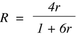
Equation 9.7 illustrates two points. First, the expected fraction of discordant
strains is dependent on only a single variable — the probability of recombination
between the two loci under analysis. In turn, since interference in any one
generation is nearly 100% over the distances analyzed by RI analysis (see
Section 7.2),
the probability of recombination can be converted directly into a
centimorgan
linkage distance (d) with an r value of 0.01 defined as equivalent to one
centimorgan. Thus:
(Equation 9.8)
![]()
Second, for values of r that are smaller than 0.01,
Equation 9.7 can be
approximated by the simpler R ~= 4r.
Thus, a 1 cM distance becomes amplified into a predicted discordance frequency of >4%. As
Taylor (1978) pointed out, this
four-fold amplification can be interpreted to mean that during RI strain
development, a locus will be transmitted, on average, through four heterozygous
animals (with four chances for a recombination event in its vicinity) before it is
fixed to homozygosity.
The amplification of the linkage map serves to enhance the usefulness of the RI approach in the analysis of closely linked loci. For example, in a group of 100 RI strains, recombination sites will be distributed at average distances of 0.25 cM, which is four times more highly resolving than that possible with an equivalent number of backcross animals. However, this same amplification has the negative consequence of limiting the usefulness of the RI approach in studying loci that are more distantly linked to each other. For example, at a distance of 25 cM (r~= 0.25), the predicted discordance level for RI strains would be 40% (R = 0.4), a value which is perilously close to the 50% expected with unlinked loci. As a consequence, the per locus swept radius obtained with RI strains will be much less than that obtainable with an equal number of backcross offspring.
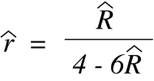
In most cases of RI analysis, an investigator wants to go from a discordance
fraction to an estimate of linkage distance. The experimentally determined
discordance fraction
R-hat
= i/Nprovides an estimate of the true value
R, which is based on the
actual probability of recombination r. By substituting
R-hat
for R in
Equation 9.7, one can
obtain a corresponding recombination fraction estimate
small r-hat.
This can be accomplished more easily if
Equation 9.7 is inverted to yield r as a function of R or, through direct
substitution,
small r-hat
as a function of
R-hat:
(Equation 9.9)
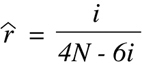
Another useful formulation of this same equation allows one to obtain the
estimated recombination fraction as a function of the sample size, N, and the
number of discordant strains, i:
(Equation 9.10)
Finally, a corresponding linkage distance estimate in centimorgans (
d-hat)
can be derived by multiplying the
small r-hat
value obtained in
Equation 9.10 by 100.
The graph in Figure 9.7 provides a rapid means for determining a linkage distance estimate from values for i and N that are commonly obtained in RI analyses. Just place a ruler over the graph so that it crosses the experimental value for N along the top and bottom axes, then observe the point at which the ruler crosses the curve associated with the experimentally-determined value for i. From this point, look across to the Y axis to read off the linkage distance in centimorgans.
Once a value for linkage distance has been obtained from RI data, the next question an investigator will ask is: how accurate is this value? The answer to this question will be critical to investigators who want to use RI data to evaluate possible relationships between the cloned gene they have just mapped and other previously mapped loci that are defined strictly in terms of a mutant phenotype. (A detailed discussion of the general strategy used to evaluate such relationships has been left to Section 9.3.4 and is illustrated in Figure 9.10.)
The accuracy of an experimentally determined value such as linkage distance can be quantitated in terms of a "confidence interval" which is defined by lower and upper boundaries — called confidence limits. To calculate a confidence interval from a body of data, one must first choose the "confidence coefficient", or level of confidence, that one wishes to attain. The confidence coefficient represents the probability with which the associated interval is likely to contain the value of the true recombination fraction or linkage distance. Each confidence coefficient will produce a different confidence interval.
In general, two particular confidence coefficients are used most often for the
evaluation of data obtained from sampling experiments aimed at estimating an
absolute real value (like linkage distance). The first is based on the standard error of
the mean:

for a normal (bell-shaped) probability distribution around a mean value:

When the lower limit of the interval around a normal distribution is set at:

and the upper limit is set at:

the corresponding confidence coefficient is always equal to 68%. It is standard practice to display
this confidence interval within a single term:
Twice as often as not, the 68% confidence interval will contain the true value being
estimated; this interval provides an investigator with an overall sense of the
accuracy of the mean estimate predicted from experimental data.
As discussed at length in Appendix D and by other authors (Silver, 1985), data obtained from linkage studies based on small sample sizes and low levels of discordance are not well approximated by "normal" probability distributions (see Figures D1 and D2). Unfortunately, the standard deviation does not provide an accurate measure of lower and upper confidence limits in the context of non-normal probability distributions (Moore and McCabe, 1989, p.41). In its place, I have used more appropriate estimates for lower and upper confidence limits associated with an actual 68% confidence interval.
The second confidence interval of critical importance for interpreting experimental data is one that encompasses the range of values likely to contain the actual recombination fraction with a probability of 95%. The more stringent 95% confidence interval is used often to define the generally accepted limits beyond which the actual value of r is unlikely to lie. A discussion of the statistical approach used to determine confidence limits for both RI strain and backcross data is presented in Appendix D along with tables of minimum and maximum values for 68% and 95% intervals. By interpolating between the numbers presented in either Table D1 or Table D2, one can derive confidence limits for pairs of i and N values generated in an analysis of 20-100 RI strains.
One special case of RI strain results deserves particular attention — when complete concordance is observed between the SDP patterns obtained for two different loci. In this special case, the Haldane-Waddington formulation (Equations 9.8 and 9.9) leads to a linkage distance estimate of 0 cM. However, if the two loci under analysis were independently-derived and known not to be identical, an estimate of zero distance clearly makes no sense. Based on intuitive grounds alone, one would expect there to be a strong likelihood that the two loci are actually separated from each other by a significant distance, especially when the total number of RI strains typed is small.
An accurate estimate of the median expected recombination fraction r-bar (leading directly to an estimate of the median expected linkage distance d-bar) that separates two completely concordant loci can be obtained by determining the midline of the area under the associated probability density function as discussed in Appendix D and illustrated in Figure D1. The results of this calculation for the range of 15 to 100 RI strains are presented graphically in Figure 9.8 along with upper limits for 68% and 95% confidence intervals.
As an example, consider the implications of these statistical formulations in the case of complete concordance between two SDP patterns for the set of 26 BXD RI strains. The median estimate of linkage distance between two concordant loci is 0.66 cM (or 1.3 megabases based on a conversion of 1 cM to 2.0 mb). The 68% confidence interval extends from 0.2 cM to 1.76 cM (or 400 kb to 3.5 megabases), and the 95% confidence interval extends from 0.02 cM to 3.95 cM (or 40 kb to 7.9 mb from the computer program presented in Appendix D). These numbers confirm the intuitive suspicion that two concordant loci typed in only a small sample set probably do not map on top of each other.
Although a small group of RI strains is not sufficient to demonstrate close linkage, this conclusion does become more appropriate as the number of concordant RI strains increases. With 100 completely concordant strains, the median estimate of linkage distance is reduced to 0.17 cM or 340 kb, the maximum limit on the 66% interval is reduced to 0.45 cM or 900 kb, and the maximum confidence limit for the 95% interval becomes 0.95 cM or 1.9 mb.
One can gain a better perspective on the accuracy of RI-determined linkage distance estimates by comparing a map obtained with the BXD set of 26 strains to a more accurate map obtained with a set of 374 backcross animals for the same eleven loci distributed over a span of 19-31 cM as shown in Figure 9.9. There are five instances here in which a single RI discordance has occurred to yield an interlocus linkage distance estimate of 1.0 cM:
with a 68% confidence interval extending from 0.7 to 3.4 cM, and a 95% interval extending from 0.2 to 6.6 cM. In three of these cases, the backcross estimate lies within the 68% confidence interval and in the other two cases, it lies within the 95% interval. There are two instances in which two RI discordances have occurred to yield an inter-locus linkage distance estimate of 2.2 cM: with a 68% confidence interval extending from 1.4 to 5.3 cM and a 95% interval extending from 0.6 to 9.6 cM. In both cases, the backcross estimate lies within the 68% interval. There are another two instances in which four RI discordances yield an interlocus linkage distance of 5.0 cM: with a 68% confidence interval extending from 3.3 to 9.7 cM, and a 95% interval extending from 1.7 to 17 cM. In one case, the backcross estimate lies within the 68% interval, and in the other case, it lies within the 95% confidence interval. Finally, there is a single instance of complete RI concordance between D17Mit10 and D17Mit6. The backcross estimate of linkage distance between these two loci lies outside the 95% confidence interval (but within the 99% confidence interval according to results obtained from the computer program listed in Appendix D).In summary, backcross estimates lie within the 68% confidence interval of the RI estimates in six (60%) of the ten pairwise comparisons, and in all but one of the remaining comparisons (90%), the backcross estimates lie within the 95% confidence interval. This level of accuracy is about as close as one can get to that predicted from statistical formulations. Furthermore, in the single case where the two mean estimates of linkage distance are significantly different from each other (0.66 cM versus 5.9 cM for D17Mit10 - D17Mit6), their associated 95% confidence intervals (0.02-3.95 cM and 3.9-8.8 cM) do overlap (barely), and the data taken together would suggest that the actual recombination frequency is somewhere between the two extreme mean values. 85
When Bailey first conceived of RI strains, it was with the notion that they would be useful for the analysis of the many forms of complex phenotypic variation that distinguish different inbred strains from each other. In the past, the use of RI strains for this purpose had been rather limited because of the absence of an overall framework of genetic markers on which phenotypic differences could be mapped. However, at present, the availability of highly polymorphic, rapidly typed DNA markers is allowing the construction of framework maps of marker loci that span essentially whole genomes in each of the major RI sets. These framework maps will finally open up RI strains to the use originally conceived of by Bailey.
There is an enormous reservoir of susceptibility differences to a variety of disease conditions, both chronic and infectious, among the classical inbred strains. For example, the A/J strain is relatively susceptible to various carcinogen-induced cancers (lung adenomas, sarcomas, and colorectal tumors), parasites (Giardia, Trypanosoma, and Plasmodium), bacteria (Listeria and Pseudomonas), viruses (Ectromelia and Herpes), and fungi (Candida albicans), as well as gall stones and teratogen-induced cleft palate; the B6 strain is relatively resistant to all of these conditions (Mu et al., 1993). On the other hand, B6 is relatively susceptible to other parasites, bacteria, viruses, and fungi as well as atherosclerosis, diabetes, and obesity; the A/J strain is relatively resistant to all of these conditions. In all, strain-specific differences in susceptibility to over 30 infectious or chronic diseases have been identified between A/J and B6, and the genetic basis for each can be approached with the use of the combined AXB/BXA set of RI strains. Differences in disease susceptibility exist among all of the traditional inbred strains, and the genes involved in many of these differences can be approached as well with the appropriate RI sets.
With most of the conditions described above, a particular genetic constitution only predisposes an individual to express a disease. This means that some individuals that carry the predisposing genotype will actually not express the disease. The fraction of genotypically identical individuals that express a particular trait defines the penetrance of that trait from that genotype. When a particular genotype guarantees the expression of a phenotype in 100% of the animals that carry it, the phenotype is considered to be completely penetrant. In all other cases, a phenotype is considered to be partially penetrant or incompletely penetrant. For example, a particular substrain of BALB/c mice is predisposed to a particular form of induced cancer known as a plasmacytoma. However, only 60% of these inbred animals actually get the cancer upon induction. Thus, the penetrance of induced- plasmacytoma in these mice is 60%.
The cousin of incomplete penetrance is variable expressivity. Variable expressivity describes the situation in which multiple individuals all express a particular trait, but in a quantitatively distinguishable manner. For example, a tumor may appear at a young age or an old age, a birth defect such as cleft palate may be more or less severe. Variable expressivity can also be measured for traits that do not show an either/or type of wild-type/mutant variation. For example, there are many strain-specific differences in physiological parameters and behavior that are strictly quantitative. Thus, blood cholesterol levels may vary among different strains as will the average number of pups that a female has in a litter (see Table 4.1).
Both incomplete penetrance and variable expressivity can be caused by genetic as well as non-genetic factors. Inbred strains allow one to clearly distinguish genetic factors since measurements can be made of the mean level of expression or penetrance of a trait in one strain relative to another when populations of both are maintained under identical environmental conditions.
In cases where two strains differ quantitatively in penetrance levels and/or expressivity for a particular trait, it becomes difficult to design traditional breeding crosses that can uncover the loci involved. For example, if strain A shows 20% penetrance for a trait and strain B shows 80% penetrance for the same trait, then its expression in offspring from a cross between the two strains would not provide straightforward information as to which predisposing allele(s) is present. In contrast, each RI strain provides an unlimited number of animals with the same homozygous genotype. Thus, through the analysis of a sufficient number of animals, it becomes possible to quantitate the levels of penetrance and expressivity and associate distinct measurements of mean and standard deviation with each RI genotype. Furthermore, it is just as easy to map recessive traits as dominant traits since RI strains are completely homozygous.
RI strains are also useful in those cases where multiple animals must be sacrificed in order to make a single phenotypic determination. This will be true for certain biochemical assays (although in most cases today, microtechniques allow analysis on tissues obtained from single animals) and for other assays that require a determination of multiple test points in which each point is a single animal. An example of the latter would be an LD50 determination for a particular toxic chemical. 86
If every RI strain in a set expresses a trait with essentially the same penetrance and expressivity as one of the two progenitor strains, and approximately half of the RI strains resemble one progenitor and half resemble the other, determining a map position for the responsible locus is no different than that described earlier in the case of DNA marker loci. Data of this type can be viewed as evidence in favor of a single major locus that is responsible for the difference in susceptibility, penetrance, or expressivity between the two progenitor strains. One can simply write out an SDP for the phenotype and then subject this SDP to concordance analysis with the SDPs obtained for all previously typed markers as described in Section 9.2.2. Once linkage is demonstrated, gene order and map distances can be determined as described in Sections 9.2.3 and 9.2.4.
There are two forms of RI strain data that are indicative of a more complex basis of inheritance which may be impossible to resolve using only the RI approach. The first occurs when there is a significant departure from a balanced SDP in that the phenotype expressed by one progenitor strain is found in many more RI strains than the alternative phenotype. Data of this type would suggest that the expression of the rarer phenotype requires the simultaneous presence of two or more genes from the appropriate progenitor. One can calculate the probability of occurrence of a phenotype that requires the action of two or more unlinked loci through the law of the product as (0.5)n, where n is the number of loci required. 87 Thus, if two unlinked B6 loci are both required for susceptibility to a particular viral infection (relative to DBA), only (0.5)2 = 25% of the BXD RI strains would be expected to show susceptibility. Unfortunately, for obvious reasons, unbalanced SDPs cannot be compared directly for linkage relationships with normal single-locus marker SDPs. 88
The second form of RI data indicative of genetic complexity is the occurrence of strains that show a level of penetrance or expressivity that is significantly different from both of the progenitors. Since every RI strain can be considered homozygous for one progenitor allele or the other at every locus, data of this type will also implicate the action of multiple genes. The simplest explanation for these results is that different combinations of alleles from the two progenitors cause the different levels of phenotypic expression. For example, with the involvement of two loci, X and Y, in the expression of a trait that distinguishes the strains A/J and B6, there will be four relevant genotypes among the AXB/BXA RI strains:
Many variations upon these examples are possible. Thus, every complex trait will have to be approached independently to formulate a reasonable hypothesis for inheritance. In some cases, RI strains may still provide an appropriate tool for genetic analysis, but in most cases, it will be necessary to move to a different form of analysis that may require the establishment of a new breeding cross as described in Section 9.4.