9.1 DEMONSTRATION OF LINKAGE AND STATISTICAL ANALYSIS
9.1.1 Mapping new DNA loci with established mapping panels
When a new mouse locus has been defined at the DNA level, it can be mapped
by three different approaches: somatic cell hybrid analysis, in situ hybridization, or
formal linkage analysis. The first of these approaches is not applicable generally to
the mouse because single chromosome hybrids have not been gathered together in a
systematic way for the whole mouse genome. However, even in those cases where
such hybrids exist, this type of analysis provides only a chromosomal assignment.
The second approach — in situ hybridization — is more highly resolving than
somatic cell hybrid analysis, but this protocol requires special expertise and the
resolution is still less than that obtained routinely with linkage analysis. Both of
these non-sexual mapping protocols have two advantages over all forms of linkage
analysis. First, they do not require any prior knowledge of map positions for other
loci. Second, they allow the mapping of non-polymorphic loci. Thus, in the early
days of mouse molecular genetics, before many DNA markers had been placed onto
the map, and before new methods for uncovering polymorphisms had been
developed, both of these protocols served useful functions in the arsenal of general
mapping tools.
Today, the method of choice for mapping a new locus defined at the DNA level
will always be formal linkage analysis. There are two interrelated reasons for this.
First, a whole genome mouse linkage map of very high density has been developed
with thousands of polymorphic DNA markers already in place and new ones being
added each month
(Copeland et al., 1993). The second reason lies within the
existence of various mouse "mapping panels" that have been established by a
number of investigators at different institutions around the world.
A mapping panel is a set of DNA samples obtained from animals that carry
random recombinant chromosomes produced within the context of a specific
breeding scheme. The most widely used mouse mapping panels are of two specific
types. One consists of representative DNA samples derived from each strain of a
recombinant inbred (RI) set or group of RI sets. The approach to mapping with RI
strains will be detailed in
Section 9.2. The second type of widely used mapping panel
contains samples derived from the offspring of an interspecific backcross between
the two species, M. musculus and M. spretus. This approach will be discussed in
Section 9.3. It is also possible to design mapping panels that are based on an
intercross between two F1 hybrid parents obtained in an interspecific or
intersubspecific outcross between two different inbred strains
(Dietrich et al., 1992).
The power of mapping panels lies within the database of information that is
already available for a large number of previously typed loci in members of the
same defined cohort of animals. The most useful panels have been typed for at least
200 independent DNA markers and, in fact, the most well-established
panels have been typed for many more. In classical genetic terminology, this can be
viewed as a multihundred point cross that provides linkage maps across the
complete spans of all chromosomes in the genome.
Thus, the mapping of a new locus can be accomplished simply by genotyping
each of the samples in the same cohort (or a subset thereof) for just the new locus of
interest. It is never necessary to type more than one hundred animals in the initial
analysis and, as discussed in
Sections
9.2 and
9.4, with a well-characterized panel, one
can usually obtain a map position with the typing of 50 or fewer animals. A single
investigator can easily carry out such an analysis in less than a week's time with the
use of either a PCR analysis or Southern blotting. The results obtained are entered
into the database containing all prior mapping information on the panel and a
computational algorithm is used to determine the location of the new locus within
the already-established linkage map. Essentially, this is accomplished by searching
for concordant segregation between alleles at the new locus and those at one or
more loci that have been previously typed on the same panel. With a well-established
mapping panel, a first-order map position will always be obtained.
A discussion of the two most important classes of mapping panels — recombinant
inbred strains and the interspecific backcross — will be presented in Sections
9.2 and
9.3 of this Chapter.
9.1.2 Anchoring centromeres and telomeres onto the map
As discussed in
Section 5.2, all 21 chromosomes in the standard mouse
karyotype (19 autosomes and the X and Y) are extremely acrocentric. Even with very
high resolution light microscopy of extended prophase chromosomes, the
centromere appears to lie at one end of each chromosome. Although there must be
a segment of DNA containing at least a telomeric sequence that precedes the
centromere, no unique sequence loci have ever been localized to this hypothetical
segment. Thus, for all intends and purposes, one can view the genetic map of each
chromosome as beginning with a centromere and ending with a telomere.
In the absence of centromere and telomere mapping information, a linkage map
will be unanchored. As a result, the length of genetic material that lies beyond the
furthermost marker at each end of the map will not be known. However, since both
centromeres and telomeres are composed of repeated simple sequences that are
shared among all chromosomes, their direct mapping requires special approaches.
9.1.2.1 Telomere mapping
All mammalian telomeres are composed of thousands of tandem copies of the
same basic repeat unit TTAGGG
(Moyzis et al., 1988;
Elliott and Yen, 1991). Early
sequence comparisons indicated that while the basic repeat unit was highly
conserved, occassional nucleotide changes could arise anywhere within the large
telomeric sequence present at the end of any chromosome.
Elliott and Yen (1991)
realized that one particular nucleotide change, from a G to a C in the sixth position
of this repeat unit, would create a DdeI restriction site (CTNAG) that overlapped two
adjacent repeats —
[TTAGGC][TTAGGG]. In the absence of such a change, the
enzyme DdeI would not cut anywhere inside a particular telomeric region which
would remain intact within a restriction fragment of 20 kb or more in size. In
contrast, one or more substitutions of the type described would allow DdeI to reduce
a telomeric region into smaller restriction fragments that could be detected by
probing a Southern blot with a labeled oligonucleotide (called TELO) consisting of
five tandem copies of the consensus telomere hexamer
(Elliott and Yen, 1991). To
date, strain-specific telomeric DdeI RFLPs have allowed the inclusion of telomeres
from six mouse chromosomes as segregating markers in linkage studies
(Eicher and Shown, 1993;
Ceci et al., 1994). More recently, another repeat sequence has been
identified with a subtelomeric position in all mouse chromosomes
(Broccoli et al., 1992). In the future, it may be possible to develop
analogous strategies for mapping telomeres with this subtelomeric repeat as well.
9.1.2.2 Centromere mapping with Robertsonian chromosomes
Unfortunately, the satellite sequences present within all mouse centromeres are
not amenable to the same type of mapping strategy just described. The problem is
that each centromere contains about eight megabases of satellite sequences
(Section 5.3.4), which is about 400 times larger than a telomere.
Consequently, base substitutions away from the consensus satellite sequence will be much more
numerous; this will lead to whole genome Southern blot patterns, with any
restriction enzyme, that are unresolvable smears.
So, how does one go about placing centromeres onto a linkage map? One
approach is to mark the centromeres of individual homologs with a Robertsonian
fusion (see
Section 5.2). If a test animal is heterozygous for a particular
Robertsonian chromosome, the segregation of the fused centromere can be followed
in each offspring through karyotypic analysis. If the Robertsonian chromosome
carries distinguishable alleles at linked loci, the recombination distance between the
centromere and these linked loci can be determined by DNA marker typing.
Unfortunately, this approach is complicated by the finding that local recombination
is suppressed in animals heterozygous for many Robertsonian chromosomes due to
minor structural differences that interfere with meiotic pairing
(Davisson and Akeson, 1993). Thus, the distance between
the centromere and the nearest genetic locus is likely to be underestimated by this method.
9.1.2.3 Centromere mapping through secondary oocytes
A second approach to determining distances between centromeres and linked
markers is based on the genetic analysis of large numbers of individual "secondary
oocytes," which are the products of the first meiotic division. As shown in
Figure 9.1,
sister chromatids remain together in the same nucleus after the first meiotic
division. Thus, in the absence of crossing over, the secondary oocyte will receive
one complete parental homolog or the other, and would appear 034;homozygous" for
all markers upon genetic analysis. However, if crossing over does occur, the oocyte
will receive both parental alleles at all loci on the telomeric side of the crossover
event. Thus, all telomeric-side loci that were heterozygous in the parent will also
appear heterozygous in the oocyte, but all centromeric-side loci will remain
homozygous. The fraction of individual oocytes that are heterozygous for a
particular genetic marker will be twice the linkage distance that separates that
marker from the centromere since only half of the haploid gametes generated from
a double allele oocyte will actually carry the recombinant chromatid.
How does one go about determining the individual genotypes of large numbers
of secondary oocytes? There are two basic protocols. The first to be developed was
based on the clonal amplification of secondary oocytes within the form of ovarian
teratomas
(Eicher, 1978). Ovarian teratomas result from the parthenogenetic
development of secondary oocytes into disorganized tumors that contain many
different cell types. The inbred LT/Sv strain of mice undergoes spontaneous
ovarian teratoma formation at a very high rate. This inbred strain in and of itself is
not useful for oocyte-based linkage analysis since it is homozygous at all loci, but it is
possible to construct congenic animals that are heterozygous for particular marker
loci within an overall LT/Sv genetic background. In the cases reported, these
congenic animals retain the high rate of teratoma formation associated with the
parental LT/Sv strain
(Eppig and Eicher, 1983;
Artzt et al., 1987;
Eppig and Eicher, 1988).
This approach is tedious in that a different congenic line has to be developed
to map centromeres on each chromosome, but there is every reason to believe that
the results obtained are an accurate measure of centromere-marker linkage distances
in female mice.
An alternative protocol for genotyping oocytes is based on DNA amplification
(by PCR) rather than cellular amplification. The main advantage to this approach is
that genotyping can be performed on oocytes derived from any heterozygous female
(Cui et al., 1992). Thus, in theory, this approach could be used to position the
centromere relative to any marker on any chromosome. However, in practice, PCR
amplification from single cells is difficult, and there is a high potential for artifactual
results — such as amplification from one DNA molecule but not its homolog.
9.1.2.4 Centromere mapping by in situ hybridization or Southern blots
A third approach to positioning centromeres on linkage maps is based on direct
cytological analysis. This approach is possible because of the divergence in
centromeric satellite DNA sequences that has occurred since the separation of
M. musculus and M. spretus from a common ancestor ~3 million years ago
(see Section 5.3 and
Figure 2.2).
In particular, the major satellite sequence in M. musculus
is composed of a 234 bp repeat unit that is present in 700,000 copies distributed
among all the centromeres. This same 234 bp repeat unit is only present in 25,000
copies spread among the centromeres in M. spretus
(Matsuda and Chapman, 1991).
The 28-fold differential in copy number can be exploited with the technique of in
situ hybridization to readily distinguish the segregation of M. musculus
centromeres from M. spretus centromeres in the offspring of an interspecific
backcross. This approach has now been used to anchor all of the mouse
chromosomes at their centromeric ends
(Ceci et al., 1994). The only caveat to
mention is the possibility that interspecific hybrids have a distorted recombination
frequency in the vicinity of their centromeres.
A final possibility, that has yet to be validated, is the mapping of centromeres as
RFLPs observed on Southern blots in the same manner as described for telomeres in
Section 9.1.2.1. This approach may be possible with the use of a newly described
repeat sequence that appears to be present in reasonable copy numbers adjacent to
the centromeres of nearly every mouse chromosome
(Broccoli et al., 1992).
9.1.3 Statistical treatment of linkage data
9.1.3.1 Testing the null hypothesis
Let us assume that two inbred strains of mice (B6 and C3H for example) carry
distinguishable alleles (symbolized by b and c respectively) at each of two fictitious
loci Xy1 and Gh3 as shown in
Figure 9.2.
An F1 hybrid between B6 and C3H will be
heterozygous at each locus with a genotype of:
Xy1c/Xy1b,
Gh3c/Gh3b
If these two
loci are linked on a single chromosome, the F1 hybrid will have one homolog with the
Xy1c and
Gh3c alleles, and the other homolog with the
Xy1b and
Gh3b alleles. By
definition, linkage means that the F1 hybrid will produce a greater number of
gametes carrying a parental set of alleles, either:
Xy1b Gh3b or
Xy1c Gh3c
than a recombinant set of alleles, either:
Xy1b Gh3c or
Xy1c Gh3b.
As discussed at length in
Section 7.2, the actual distance that separates the two loci will determine the strength
of their linkage in terms of the fraction of recombinant gametes.
If one could determine the haploid genotype (or
haplotype) of each sperm
produced by a C3H X B6 hybrid male, one would know for sure whether the two loci
in question are linked. But with the typing of a finite number of progeny in an
experimental cross, the answer is often not as clear. Let us say that 100 offspring
from the F1 hybrid have been typed to test for linkage between Xy1 and Gh3 with the
result that 62 carry parental allele combinations and 38 carry non-parental allele
combinations. Do these data provide evidence in favor of the hypothesis: "Xy1 and
Gh3 are linked"?
Unfortunately, there is a problem with a general hypothesis that states "genes A
and B are linked" in that there is no precise prediction of what to expect in terms of
data from a breeding experiment. This is because linkage can be very tight so that
recombination would be expected rarely, or linkage can be rather loose so that
recombination would be expected frequently. Of course, the strength of linkage, if
indeed the genes under analysis are linked, is unknown at the outset of the
experiment. In contrast, there is a precise prediction of what to expect from the so-
called "null hypothesis" of no linkage between genes A and B. The prediction of
this null hypothesis is that alleles at different genes will assort independently
leading to a 50:50 ratio of gametes with parental or recombinant combinations of
alleles.
Thus, whenever geneticists wish to determine whether their data provide
evidence for linkage (of any degree), what they actually do is ask the following
question: are these data significantly different from what one would expect if the
two loci were not linked? With this well-defined "null hypothesis", it becomes
possible to apply a statistical test to determine whether the data actually observed are
significantly different from the expected outcome for no linkage. In the example
above, with the analysis of 100 offspring, the null hypothesis would lead to a
prediction of 50 animals with a parental allele combination and 50 animals with a
recombinant allele combination in comparison with the observed results of 62 and
38 respectively. Are these two sets of numbers significantly different from each
other? If the answer is yes, this would suggest that the null hypothesis is false and
that the two loci are indeed linked. On the other hand, if the observed data are not
significantly different from those expected from the null hypothesis, the question of
linkage will remain unresolved — the two loci may be unlinked, but it may also be
possible that the loci are linked and there are simply not enough data to detect it.
9.1.3.2 A comparison of mouse linkage data and human pedigree data
Before launching into a discussion of the statistical treatment of linkage data, it is
important to illuminate a critical difference between linkage analysis in the mouse
and in humans. In nearly all cases of linkage analysis in the mouse, the parental
combinations of alleles — the so-called phase of linkage — will be known with
absolute certainty. In the example above, if we assume that the two loci in question
are linked, we know that the
Xy1c and
Gh3c alleles will be present on one homolog and the
Xy1b and
Gh3b alleles will be present on the other homolog in the F1 hybrid,
as illustrated in
Figure 9.2.
With this information, we can tell immediately upon
typing whether an offspring carries a parental or recombinant combination of
alleles.
More often than not, the phase of linkage is not known with certainty in the
analysis of human pedigrees. As a consequence, human geneticists are forced to
employ more sophisticated statistical tools that evaluate results in light of the
probabilities associated with each possible phase relationship for each parent in a
pedigree
(Elston and Stewart, 1971).
These maximum likelihood estimation (MLE)
analyses are always performed by computer and they lead to the determination of
LOD score graphs which show the likelihood of linkage between two loci over a
range of map distances
(Morton, 1955). With most human pedigrees, it is
impossible to count the actual number of recombination events that have occurred
between two loci, and, as a consequence, it is impossible to determine even a most
likely genetic distance separating two loci without the use of a computer. In
contrast, all recombination events can be clearly detected in two of the three most
common types of mouse breeding protocols — the backcross and RI strains — and
with the intercross, all but a small percentage of recombination events can also be
distinguished unambiguously (see
Figure 9.4).
With backcross and RI data in
particular, linkage distance estimates can be easily determined by hand or with a
simple calculator, and confidence limits around these estimates can be extrapolated
from sets of tables (such as those in
Appendix D).
9.1.3.3 The
Chi-squared
test for backcross data
The standard method for evaluating whether non-Mendelian recombination
results are statistically significant is the "method of
Chi-squared."
Upon calculating a value for
Chi-squared,
one can use a look-up table to determine the likelihood that an observed set of
data represents a chance deviation from the values predicted by a particular
hypothesis. This determination can lead one to reject or accept the hypothesis that is
being tested.
In its most general form, the
Chi-squared
statistic is defined as follows:
(Equation 9.1)
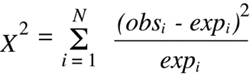
where there are n potential outcome classes, each of which is associated with an
observed number (obsi) that is experimentally determined and an expected number
(expi) that is calculated from the hypothesis being tested. It is obvious from a quick
examination of
Equation 9.1 that as the differences between observed and expected
values become larger, the calculated value of
Chi-squared
will also become larger. Thus the
Chi-squared
value is inversely related to the goodness of fit between the experimental results
and the null hypothesis being tested, with a
Chi-squared
value of zero indicating a perfect fit. As the value of
Chi-squared
grows larger and larger, the likelihood that the experimental data
can be explained by the null hypothesis becomes smaller and smaller.
Consider the case of a backcross with the (B6 X C3H) F1 hybrid described above to
analyze the possibility of linkage between the fictitious loci Xy1 and Gh3. In terms of
these two loci, the F1 hybrid can produce four types of meiotic products which will
engender four experimental outcome classes (
Figure 9.2).
If one makes the a priori
assumption that the two parental classes represent different manifestations of the
same outcome of no recombination, and the two other classes represent, for all
practical purposes, reciprocal products of the same recombination event, then the
data can be reduced in complexity to a set of just two outcomes — parental or
recombinant.
69
In this case, the
Chi-squared
statistic becomes:
(Equation 9.2)
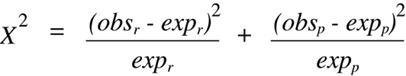
where the r subscript indicates recombinant and the p subscript indicates parental.
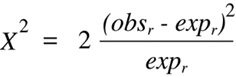
Whenever the
Chi-squared
test is used to analyze data obtained from a backcross and the
null hypothesis is one of no linkage, a further simplification of
Equation 9.2 can be
accomplished. In this case, the expected values for parental and recombinant classes
will both be equivalent to half the total number (N) of offspring typed (which is the
sum of the two observed values). Furthermore, the two observed values will both
differ from the expected value by the same absolute number, and the square of each
difference will yield the same positive value. Thus, the two terms in
Equation 9.2
can be combined to form:
(Equation 9.3)
Equation 9.3 can be simplified even further by substituting each appearance of expr
with the equivalent expression (obsp + obsr)/2. The form of the equation that is so derived
contains only the two experimentally obtained values as variables:
(Equation 9.4)
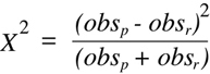
In plain English,
Equation 9.4 can be read as "square the difference, divide by the
sum",; and this simple calculation can often be performed through mental
calculations alone.
70
Now we can return to our example from above with 62 parental and 38
recombinant allele combinations and use
Equation 9.4 to determine the appropriate
Chi-squared
value. The difference between the numbers in the two observation
classes (62 - 38 = 24) is squared to yield 576, and this value is divided by the total size of the sampled
population (100) to yield 5.76.
One more piece of information is required before it is possible to translate a
Chi-squared
value into a measurement of significance — the number of "degrees of freedom" (df)
associated with the particular experimental design. The "degrees of freedom" is
always one less than the total number of potential outcome classes (df = n - 1). The
rationale for this definition is that it is always possible to determine the number of
events that have occurred in the any one class by subtracting the sum of the events
in all other classes from the total size of the sample set. In the backcross example
under discussion, we have defined two potential outcome classes: recombinant and
parental. Knowing the number in either class, along with the total sample size,
provides the number in the other class. Thus, the number of degrees of freedom in
this case is one.
With a
Chi-squared
value and the number of degrees of freedom in hand, one can proceed to a
Chi-squared
probability look-up table such as the one presented in
Table 9.1.
This table shows the
Chi-squared
values that are associated with different "P values." A P value is a
measure of the probability with which a particular data set, or one even more
extreme, would have occured just by chance if the null hypothesis were indeed true.
To obtain a P value for the data set in the example under discussion, we would look
across the row associated with one degree of freedom to find the largest
Chi-squared
value that is still less than the one obtained experimentally. In this case, this procedure yields the
Chi-squared
value of 3.8. Looking up the column from this
Chi-squared
value, we obtain a P value of 0.05.
71
We have now reached the final goal of our statistical test for significance.
In this hypothetical example, our statistical analysis indicates that the data
obtained would be expected to occur with a frequency of less than 5% if the two loci
were not linked. However, is this result significant enough to prove linkage? To answer
this question, it is very important to understand exactly what it is that the
Chi-squared
test and its associated P value do and what they do not do. The outcome of a
Chi-squared
test cannot prove linkage or the absence thereof. It just provides one with a quantitative
measure of significance. What is a significant result? Traditionally, scientists have
chosen a P value of 0.05 as an arbitrary cutoff. But with this choice, one will
conclude falsely that linkage exists in one of every twenty experiments conducted on
loci that are, in fact, not linked! As discussed below in
Section 9.1.3.6, the interpretation of a
Chi-squared
value in modern genetic experiments that look
simultaneously for linkage between a test locus and large numbers of genetic
markers is subject to further restrictions that result from the application of Bayes'
theorem.
9.1.3.4 The
Chi-squared
test for intercross data
It is instructive to consider the application of the
Chi-squared
test to a breeding protocol with more than two potential outcome classes. The most relevant example of this
type is the intercross between two F1 hybrid animals that are identically
heterozygous at two loci with a genotype of A/a, B/b.
Figure 9.3
illustrates the
different types of F2 offspring genotypes that are possible in the form of a Punnett
square. In the absence of linkage between A and B one would expect each of the
sixteen squares shown to be represented in equal proportions among the F2 progeny.
If one compares the actual genotypes present in each square, one finds that there is
some redundancy with only nine different genotypes in total. These are as follows
(with their relative occurrences in the Punnett Square shown in parenthesis):
- A/A, B/B (1)
- a/a, b/b (1)
- A/a, B/b (4)
- A/A, B/b (2)
- A/a, B/B (2)
- A/a, b/b (2)
- a/a, B/b (2)
- A/A, b/b (1)
- a/a, B/B (1)
However, as in the case of the backcross, these classes are
not really independent of each other. In particular, two classes:
result from the transmission of parental allele combinations from both F1
parents (zero recombinants in
Figure 9.4),
four classes:
- A/A, B/b
- A/a, b/b
- a/a, B/b
- A/a, B/B
result from a single recombination event in one parent or the other,
two classes result from two recombination events:
and the final class (A/a, B/b) is ambiguous and could result from either no recombination in
either parent or recombination events in both parents. Thus, the the nine genotypic
outcomes from the double heterozygous intercross can be combined into four truly
independent genotypic classes. By adding up the number of squares included within
any one class and dividing by the total (16), one obtains the fraction of offspring
expected in each in the case of the null hypothesis:
- zero recombinants — 1/8
- single recombinants — 1/2
- double recombinants — 1/8
- ambiguous (zero or two recombinants) — 1/4
As discussed above, four outcome classes yield three degrees of
freedom.
With this information, it becomes possible to set up a
Chi-squared
test to evaluate the evidence for linkage between two segregating loci typed among the progeny of an
(F1 X F1) intercross. The special
Chi-squared
equation for the intercross takes the following
form:
(Equation 9.5)
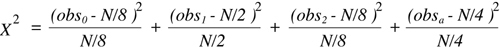
where the subscript in each observational class indicates the number of
recombination events (obsa is the ambiguous class) and N is the total number of F2
progeny typed. An comparison of the experimentally determined
Chi-squared
value with the critical values shown in the df = 3 row of
Table 9.2
will allow a determination of a corresponding P value.
9.1.3.5 Limitations and corrections in the use of the
Chi-squared test
The
Chi-squared
test does have some limitations in usage. First, it cannot be applied to
very small data sets, which are defined as those in which 20% or more of the
outcome classes have expected values that are less than five
(Cochran, 1954). With
this rule, it is possible to set minimum sample sizes required for the analysis of
backcross data at 10, and F1 X F1 intercross data at 40. In actuality, a backcross or RI
data set must include at least 13 samples to show significance in the case of no
recombinants (based on the Bayesian correction described below). Furthermore,
when the sample size is below 40 (in cases of one degree of freedom only), a more
accurate P value is obtained if one includes the Yates correction for small numbers.
This is accomplished by subtracting 0.5 from the absolute difference between
observed and expected values in the numerator of
Equation 9.3.
A final point is that
Chi-squared
analysis provides a general statistical test for significance
that can be used with many different experimental designs and with null
hypotheses other than the complete absence of linkage. As long as a null hypothesis
can be proposed that leads to a predicted set of values for a defined set of data classes,
then one can readily determine the goodness of fit between the null hypothesis and
the data that are actually collected.
9.1.3.6 A Bayesian correction for whole genome linkage testing
If one has reason to believe from other results that two loci are just as likely to
be linked as not, then the P value obtained with the
Chi-squared
test can be used directly as an
estimate of the probability with which the null hypothesis is likely to be true, and
subtracting the P value from the integer one provides a direct estimate of the
probability of linkage. However, when a previously unmapped locus is being tested
for linkage to a large number of markers across the genome, there is usually no a
priori reason to expect linkage between the new locus and any one particular marker
locus. If we assume a particular experimental design such that linkage is detectable
out to 25 cM on both sides of an unmapped locus
72
and a total genome length of
1,500 cM, then the fraction of the genome in linkage with the novel locus will be
(25 + 25)/1,500 ~= 0.033. In other words, out of 100 markers distributed randomly
across the genome, one would expect only 3.3 to actually be in linkage with any
particular test locus. But, if one accepts a P value of 0.05 as providing evidence for
linkage, then 5% of the unlinked 97 loci — or an additional ~5 loci — will be falsely
considered linked according to this statistical test. As a consequence, the expected
number of false positives — five — is larger than the expected number of truly linked
loci — 3.3. Thus, of the 8.3 positive markers expected, only 3.3 would be linked, and
this means that a P value of 0.05 has only provided a probability of linkage of 40%.
This situation is clearly unacceptable.
The logical approach just discussed is referred to as Bayesian analysis after the
statistician who first suggested that prior information on the likelihood of outcomes
be included in calculations of probabilities. One can generalize from the example
given to obtain a Bayesian equation for converting any P value obtained by
Chi-squared
analysis of recombination data into an actual estimate of the probability of linkage:
73
(Equation 9.6)
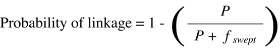
where P is the P value obtained by
Chi-squared
analysis and fswept is the fraction of the
genome over which linkage can be detected based on the power of the genetic
approach used.
74
Solutions to
Equation 9.6 for some critical P values and genomic
distances are given in
Table 9.2.
Of interest are the P values required to provide
evidence for linkage with 95% probability. So long as the experimental design allows
detection of linkage out to 15 cM, one can use a cutoff P value of 0.001 as evidence
for linkage between any two loci. In accepting linkage at P < 0.001, one is actually
setting a limit for accepting less than one false positive result for every 20 true
positive results. Later in this chapter, the Bayesian approach is used to calculate
cutoff values for the demonstration of linkage with 95% probability in the case of RI
strain data
(Figure 9.5)
and backcross data
(Figure 9.13).