(Equation D1)
To illustrate the statistical approach used to estimate confidence limits on experimentally-determined values for linkage distances, it is useful to first consider the special case where two linked loci show complete concordance or no recombination (symbolized as R = 0) in their allelic segregations among a set of N samples derived either from recombinant inbred (RI) strains or from the offspring of a backcross. Let us define the true recombination fraction — Theta — as the experimental fraction of samples expected to be discordant (or recombinant) when N approaches infinity. Then the probability of recombination in any one sample is simply Theta and the probability of non-recombination, or concordance, is simply (1 - Theta). As long as multiple events are completely independent of each other, one can calculate the probability that all of them will occur by multiplying together the individual probabilities associated with each event. Thus, if the probability of concordance in one sample is (1 - Theta), then the probability of concordance in N samples is: (1 - Theta) N.
In most experimental situations, the known and unknown variables are reversed in
that one begins by determining the number of discordant (or recombinant) samples i
that occur within a total set of N as a means to estimate the unknown true recombination fraction
Theta.
When no discordant samples are observed, the probability term just derived
can be used with the substitution of the random variable
small-theta
in place of
Theta,
to provide a
continuous probability density function indicative of the relative likelihoods for
different values of
Theta
between 0.0 (complete linkage) and 0.5 (no linkage).
(Equation D1)
![]()
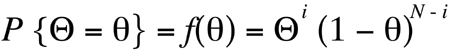
This equation reads "the probability that the true recombination fraction
Theta
is equal
to a particular value
small-theta
is the function of
small-theta
given as the last term in the equation". For
both RI data and backcross data,
Theta
can be related directly to linkage distance in
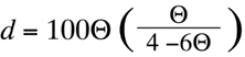
centimorgans, d. In the case of backcross data, and for values of
Theta
less than 0.25 (see
Section 7.2.2.3), recombination fractions are converted into centimorgan estimates
through simple multiplication:
(Equation D2)
![]()
In the case of RI data, this conversion is combined with the Haldane-Waddington equation
(Equation 9.8) to yield:
(Equation D3)
An example of the probability density function associated with the experimental observation of complete concordance among 50 backcross samples is shown in Figure D1. Each value of N will define a different function, but in all cases, the curve will look the same with only the steepness of the fall-off increasing as N increases. In all cases, the "maximum likelihood estimate" for the true recombination fraction Theta-hat — defined as the value of Theta associated with the highest probability — will be zero. However, since this maximum likelihood value is located at one end of the probability curve, it does not provide a useful estimate for the likely linkage distance. A better estimate would be the value of Theta which defines the midpoint below which and above which the true recombination fraction value is likely to lie with equal probability; this is the definition of the median recombination fraction estimate Theta. In mathematical terms, the value of Theta is defined at the line which equally divides the area of the complete probability density given by Equation D1 (see Figure D1).
Confidence limits are also defined by circumscribed portions of the entire probability density; the portion that lies outside a confidence interval is called alpha. For example, in the case of a 95% confidence interval, alpha = (1 - 0.95) = 0.05. It is standard practice to assign equal portions of alpha to the two "tails" of the probability density located before and after the central confidence interval. Thus, the lower confidence limit is defined as the value of small-theta bordering the initial alpha/2 fraction of the area under the entire probability curve. The upper confidence limit is defined as the value of small-theta that borders the ultimate alpha/2 fraction of the area under the entire probability curve; this is equivalent to saying that a "(1 - alpha/2)" fraction of area lies ahead of the upper confidence limit.
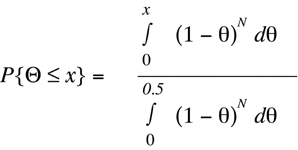
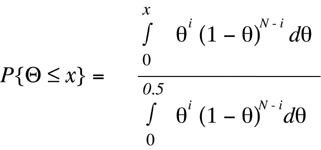
In mathematical terms, the area beneath the entire probability density curve is equal
to the definite integral of
Equation D1 over the range of legitimate values for
small-theta
between 0.0 and 0.5. To determine the fraction of the probability density that lies in the region between
Theta
= 0 and any arbitrary
Theta
= x, it is necessary to integrate over the
probability density function
(Equation D1) between these two values, and divide the
result by the total area covered by the probability density. This provides the probability
that the true recombination fraction is less than or equal to x.
(Equation D4)
By standard methods of calculus,
Equation D4 can be reduced analytically to the
form:
(Equation D5)
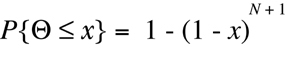
And this equation can be reformulated to yield x as a function of P{
Theta
<= x} .
(Equation D6)
![]()
By solving
Equation D6 for different values of:
P{
Theta
<= x},
one can obtain critical values of x that define the median estimate of the recombination fraction from:
P{
Theta
<= x} = 0.5,
lower confidence limits from:
P{
Theta
<= x} =
alpha/2,
and upper confidence limits from:
P{
Theta
<= x} = (1 -
alpha
/2).
Once a solution for x has been obtained, it can be converted into a linkage distance value with either
Equation D2 for backcross data or
Equation D3 for RI strain data. Solutions to
Equation D6 over a
range of N RI strains and backcross animals are shown in
Figure 9.8,
Figure 9.16, and
Figure 9.17.
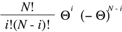
The statistical approach described above can be generalized to any case of i
discordant (or recombinant) samples observed among a total of N RI strains or
backcross animals that have been typed for two loci. As in the special case above, one
can arrive at a probability for the occurrence of multiple events by multiplying together
the individual probabilities for each event. In the general case, there will be i events of
discordance, each with an individual probability equal to the true recombination fraction
Theta,
and (N - i) events of concordance, each with an individual probability of (1 -
Theta).
These terms are multiplied together along with a "binomial coefficient" that counts
the the permutations in which the two types of events can appear to produce the
"binomial formula":
(Equation D7)
When the true recombination fraction is known, the binomial formula can be used
to provide the probability that i events of discordance will be observed in any set of N
samples. But once again, the situation encountered by geneticists is usually the reverse
one in which i and N are discrete values determined by the experiment and the true
recombination fraction
Theta
is unknown. In this case, one can substitute the random variable
small-theta
in place of
Theta
in
Equation D7 to generate a probability density function that
provides relative likelihoods for different values of
Theta
between 0.0 (complete linkage)
and 0.5 (no linkage). In this use of the binomial formula, the factorial fraction (known
as the binomial coefficient) remains constant for all values of
small-theta
and can be eliminated
since the purpose of the function is to provide relative probabilities only:
(Equation D8)
An example of the probability density function associated with the experimental observation of one discordant RI strain among a total of 26 samples is shown in Figure D2. As one can easily see, the distribution is highly skewed toward higher recombination fractions. Each discrete pair of values i and N will define a different function. When both i and N are large, the density function will approximate a normal distribution. However, with the results typically obtained in contemporary mouse linkage studies, the density function is likely to be significantly skewed as shown in Figure D2 and as such, it is usually not possible to take advantage of the simplified statistical tools developed specially for use with the normal distribution.
A median estimate of linkage distance as well as lower and upper confidence limits
can be obtained in the same manner described in the special case of no recombination
described above. This can be accomplished by substituting
Equation D8 in place of the
two occurrences of
Equation D1 within
Equation D4:
(Equation D9)
The general form of the integral in this equation cannot be solved analytically but a
short computer program can be used to estimate solutions and provide critical values of
x for defined probability values. The computer program has been written to generate
minimum and maximum values in terms of centimorgan distances for discrete
experimentally determined values of i and N from either backcross or RI data. The
program was used to generate the values shown in
Table D1,
Table D2,
Table D3,
Table D4,
Table D5, and
Table D6
for 68% and 95% confidence intervals, but it is possible to generate confidence limits
for any other integer percentile confidence interval as well. The program will also calculate
maximum likelihood and median estimates of linkage distance
109.
It is listed below as a self-contained unit that should be ready for compiling with any standard C compiler on
any computer. DOS and Macintosh version of the executable program can be downloaded over the internet from the following anonymous FTP site:
bioweb.princeton.edu.
Interested investigators should look in the folder entitled pub/mouse.
/*** A C program for the calculation of linkage distance estimates and confidence intervals ***/ #includedouble Pin(double r,int i,int N); double pow(double x, double y); double convert(double r); static int crosstype; main() { FILE *fopen(), *file; int i = 1, istart = 1, ifin = 50, iinc = 1, N = 100, P; char input; double Pin(), dmin, dmax, r,rtop, dmean, smean, Nrmlize = 0.0, Sum = 0.0, convert(), min, max; while(1){ printf("Enter the type of cross:1 for backcross,2 for RI analysis,or 3 to quit:"); scanf("%d",&crosstype); if(crosstype ! = 2 && crosstype != 1) exit(0); printf("Enter the confidence level as an integer number(e.g. 95 for 95%%):"); scanf("%d", &P); min = (1-((double)P/100.0))/2; max = 1- min; printf("Enter with comma delimiters->i-start,i-end,i-increment,and N,then return\n:>"); scanf ("%d,%d,%d,%d", &istart,&ifin,&iinc,&N); printf(" i, dist / medn, min. / max. (values in cM assuming complete interference)\n"); for ( i = istart; i <= ifin ; i += iinc){ for ( r = .0001, Nrmlize = 0 ; r <.5 ; r += .0001) Nrmlize += Pin(r,i,N); for ( r = .0001, Sum = 0; Sum < min && r<.5; r += .0001) Sum += Pin(r,i,N)/Nrmlize; dmin = convert(r); for (; Sum <.5 && r<.5; r += .0001) Sum += Pin(r,i,N)/Nrmlize; dmean = convert(r); for (; Sum < max && r<.5 ; r += .0001) Sum += Pin(r,i,N)/Nrmlize; dmax = convert(r); smean = convert((double)i/N); printf("%3d, %4.1f / %4.1f, %4.1f / %4.1f\n",i,smean,dmean,dmin,dmax);} }} double convert(double r) { double rmean; int x = 0; if(crosstype == 1) return(100*r); if(crosstype == 2) return( r*100/(4 - 6*r) );} double Pin(double r,int i,int N) { double pow(); return ((pow(r,i))*(pow(1-r,N-i)));} /************************ END OF PROGRAM ***********************/
How does one determine whether two populations of animals defined by different
inbred strains are showing a significant difference in the expression of a trait? The
answer is with a test statistic known as the "t-test" or "Student's t-test". To apply this
test, one needs to use a pair of only three values derived from an analysis of the
expression of the trait in sets of animals from each inbred strain. First is the number of
animals examined in each inbred set (N1 and N2). Second is the mean level of
expression for each set (m1 and m2) calculated as:
(Equation D10)
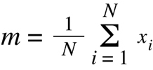
where xi refers to the expression value obtained for the ith sample in the set. Third
is the variance of each set of animals (s12 and s22) calculated as:
(Equation D11)
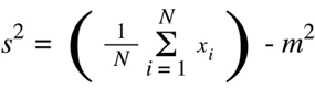
With values for the variance of each sample set and the size of each set, one can
calculate a combined parameter refered to as the "pooled variance":
(Equation D12)

Finally, one can use the value obtained for the pooled variance together with the
samples sizes and sample means to obtain a "t value":
(Equation D13)
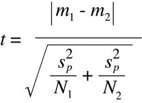
One final combined parameter is required to convert the t value into a level of
significance — the number of degrees of freedom df.
(Equation D14)
![]()
With values for t and df, one can obtain a P value from a table of critical values for
the t distribution found in
Table D7.